

Lancichinetti-Fortunato-Radicchi (N_mfl = 301)
This page shows the differences in the dynamics between the microscopic and the kinetic (meanfield) model for Lancichinetti-Fortunato-Radicchi (LFR) type graphs, depending on two parameters:
- $\sigma^2$, which is the variance of the $\beta$ distributions making up the initial distribution $f$,
- $\mu$, the so-called mixing parameter for the construction of the LFR graphs.
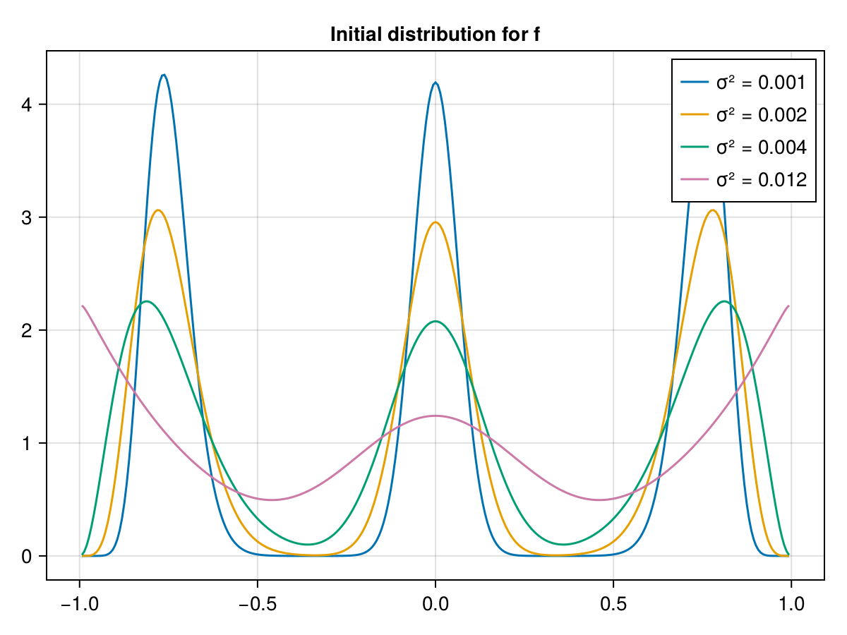
$β$ distribution with $σ² = 0.001$
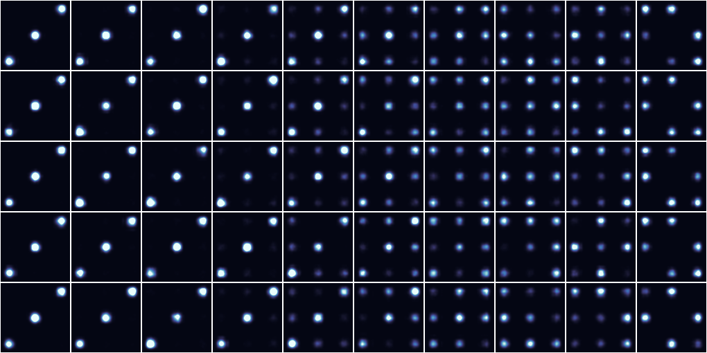
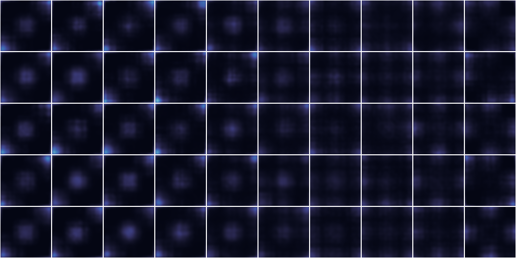
Movies (ensemble averages)
| R1 | μ=0.001 | μ=0.005 | μ=0.01 | μ=0.05 | μ=0.2083 | μ=0.3667 | μ=0.525 | μ=0.6833 | μ=0.8417 | μ=1.0 |
Graphs
Dynamics
Convergence rates are computed over the time span marked in blue in the first plot.
Parameters:
- $\mu$: LFR mixing parameter
- $T^*$: time to consensus = $-1/\log(\vert\lambda_2\vert) \cdot \delta t$, where $\lambda_2$ is the second largest eigenvalue of the transition matrix for the associated time discrete model. See here.
- assortativity
- clustering coeff.

Graph properties

g(t=0), 1 row per run, p increasing →
1
$β$ distribution with $σ² = 0.002$
Movies (ensemble averages)
| R1 | μ=0.001 | μ=0.005 | μ=0.01 | μ=0.05 | μ=0.2083 | μ=0.3667 | μ=0.525 | μ=0.6833 | μ=0.8417 | μ=1.0 |
Graphs
Dynamics
Convergence rates are computed over the time span marked in blue in the first plot.
Parameters:
- $\mu$: LFR mixing parameter
- $T^*$: time to consensus = $-1/\log(\vert\lambda_2\vert) \cdot \delta t$, where $\lambda_2$ is the second largest eigenvalue of the transition matrix for the associated time discrete model. See here.
- assortativity
- clustering coeff.

Graph properties

g(t=0), 1 row per run, p increasing →
1

$β$ distribution with $σ² = 0.004$
Movies (ensemble averages)
| R1 | μ=0.001 | μ=0.005 | μ=0.01 | μ=0.05 | μ=0.2083 | μ=0.3667 | μ=0.525 | μ=0.6833 | μ=0.8417 | μ=1.0 |
Graphs
Dynamics
Convergence rates are computed over the time span marked in blue in the first plot.
Parameters:
- $\mu$: LFR mixing parameter
- $T^*$: time to consensus = $-1/\log(\vert\lambda_2\vert) \cdot \delta t$, where $\lambda_2$ is the second largest eigenvalue of the transition matrix for the associated time discrete model. See here.
- assortativity
- clustering coeff.

Graph properties

g(t=0), 1 row per run, p increasing →
1

$β$ distribution with $σ² = 0.012$
Movies (ensemble averages)
| R1 | μ=0.001 | μ=0.005 | μ=0.01 | μ=0.05 | μ=0.2083 | μ=0.3667 | μ=0.525 | μ=0.6833 | μ=0.8417 | μ=1.0 |
Graphs
Dynamics
Convergence rates are computed over the time span marked in blue in the first plot.
Parameters:
- $\mu$: LFR mixing parameter
- $T^*$: time to consensus = $-1/\log(\vert\lambda_2\vert) \cdot \delta t$, where $\lambda_2$ is the second largest eigenvalue of the transition matrix for the associated time discrete model. See here.
- assortativity
- clustering coeff.

Graph properties

g(t=0), 1 row per run, p increasing →
1